Wasserstein GANs
The Wasserstein GAN (WGAN) is a recent algorithm developed by researchers at Facebook AI Research for Generative Modeling using Generative Adversarial Networks (GANs). If you don’t know what Generative Models or GANs are all about, here is a great post by OpenAI explaining why Generative Modeling is so crucial to AI and how GANs can be used for it. This rather short post is about how WGANs work without the technical (but beautiful!) details.
Like all other generative models, the goal of WGANs is to learn a probability distribution \(P_{\theta}\) that approximates the real distribution of data, \(P_{r}\), as closely as possible. To do this we first need to find a way to measure how far away \(P_{\theta}\) is from \(P_{r}\). WGANs use the Wasserstein-1 to measure the distance between probability distributions and it is defined as follows:
\[\mathbb{W}(P_{r}, P_{\theta}) = \underset{w \in W}{\text{max}}\quad \mathbb{E}_{x_{real} \sim P_{r}}(f_{w}(x_{real})) - \mathbb{E}_{x_{fake} \sim P_{\theta}}(f_{w}(x_{fake}))\]Where, \(f_{w}\) is the ‘critic’ function with parameters \(w\). However, \(f_{w}\) cannot be just any function, it must be \(K\)-Lipschitz, fortunately, we can make it so just by restricting \(w\) within a particular set of possible values \(W\). So what is going on up there? The above equation just says that the distance between the two distribution \(P_{r}\) and \(P_{\theta}\) is equal to the maximum over \(w\) of the difference between the expectation of \(f_{w}(x_{real})\) and \(f_{w}(x_{fake})\). Different values of \(w\) would give us different values for this difference. We have to find the \(w_{max}\) that maximizes it (but is within \(W\)) to find the correct distance between the two distributions. Once the correct distance is found we can tweak the parameters of \(P_{\theta}\) so that we can reduce it.
As with GANs, \(x_{fake}\) is generated by sampling a random vector, \(z\), from a prior distribution, \(p_{z}\) (usually gaussian), and passing it through a neural network, \(g_{\theta}\), with parameters \(\theta\) which can be learnt.\(^{*}\) Therefore, we get that \(x_{real} = g_{\theta}(z)\) or \(P_{\theta} = g_{\theta}(z)\). The function \(f_{w}\), too can be modelled as a neural network with parameters \(w\) such that \(w \in W\).
\(^{*}\)Technical Note: \(g_{\theta}\) cannot be just any neural network, it must be one consisting of affine transformations and nonlinearities which are smooth Lipschitz functions (e.g ReLU, Sigmoid, Tanh, elu, softplus). This means that most standard neural network architectures work just fine.
The Algorithm
The algorithm for training the WGAN is given below:
- Initial Parameters: \(w_{0}\): initial parameters of \(f_{w}\), \(\theta_{0}\): initial parameters of \(g_{\theta}\), \(n_{critic}\): the number of maximization iterations of \(f_{w}\) per generator iteration, \(m\): batch size, \(\alpha\): learning rate, \(c\): clipping parameter
while \(\theta\) has not converged do
for \(t = 0, \dots, n_{critic}\) do
Sample {\(x_{real}^{(i)}\)} \(\sim P_{real}\) a batch of real samples
Sample {\(z^{(i)}\)} \(\sim p(z)\) a batch of priors
Calculate gradient w.r.t \(w\):\(\quad \mathcal{G}_{w} \leftarrow \nabla_{w} \left[\frac{1}{m}\sum\limits_{i = 1}^{m}f_{w}(x_{real}^{(i)}) - \frac{1}{m}\sum\limits_{i = 1}^{m}f_{w}(g_{\theta}(z^{(i)}))\right]\)
Update \(w\):\(\quad w \leftarrow w + \alpha \times \text{RMSProp}(w, \mathcal{G}_{w})\)
Clip \(w\):\(\quad w \leftarrow \text{clip}(w, -c, c)\)
end for
Sample {\(z^{(i)}\)} \(\sim p(z)\) a batch of priors
Calculate gradient w.r.t \(\theta\): \(\quad \mathcal{G}_{\theta} \leftarrow \nabla_{\theta} \left[\frac{1}{m}\sum\limits_{i = 1}^{m}f_{w}(x_{real}^{(i)}) - \frac{1}{m}\sum\limits_{i = 1}^{m}f_{w}(g_{\theta}(z^{(i)}))\right]\)
Update \(\theta\):\(\quad \theta \leftarrow \theta - \alpha \times \text{RMSProp}(\theta, \mathcal{G}_{\theta})\)
end while
In every epoch we first find the distance between the distribution generated by \(g_{\theta}(z)\) and the real distribution \(P_{r}\) by finding the \(w\) that maximizes \(\left[\frac{1}{m}\sum\limits_{i = 1}^{m}f_{w}(x_{real}^{(i)}) - \frac{1}{m}\sum\limits_{i = 1}^{m}f_{w}(g_{\theta}(z^{(i)}))\right]\) (lines 2 - 6). We then clip the updated \(w\) to ensure \(f_{w}\) is \(K\)-Lipschitz. Once the correct distance is learnt we fix \(w\) and update \(\theta\), the parameters of \(g_{\theta}\), to minimize this distance (lines 9 - 10). We repeat this process till convergence is reached.
Empirical Results
The results here are right from the WGAN paper. Perhaps the most important property the authors found of WGANs
is that the Wasserstien-1 distance correlates quite well with sample quality. Figures 1 and 2 give two examples of WGANs trained with different
architecutres on the LSUN-Bedrooms dataset.
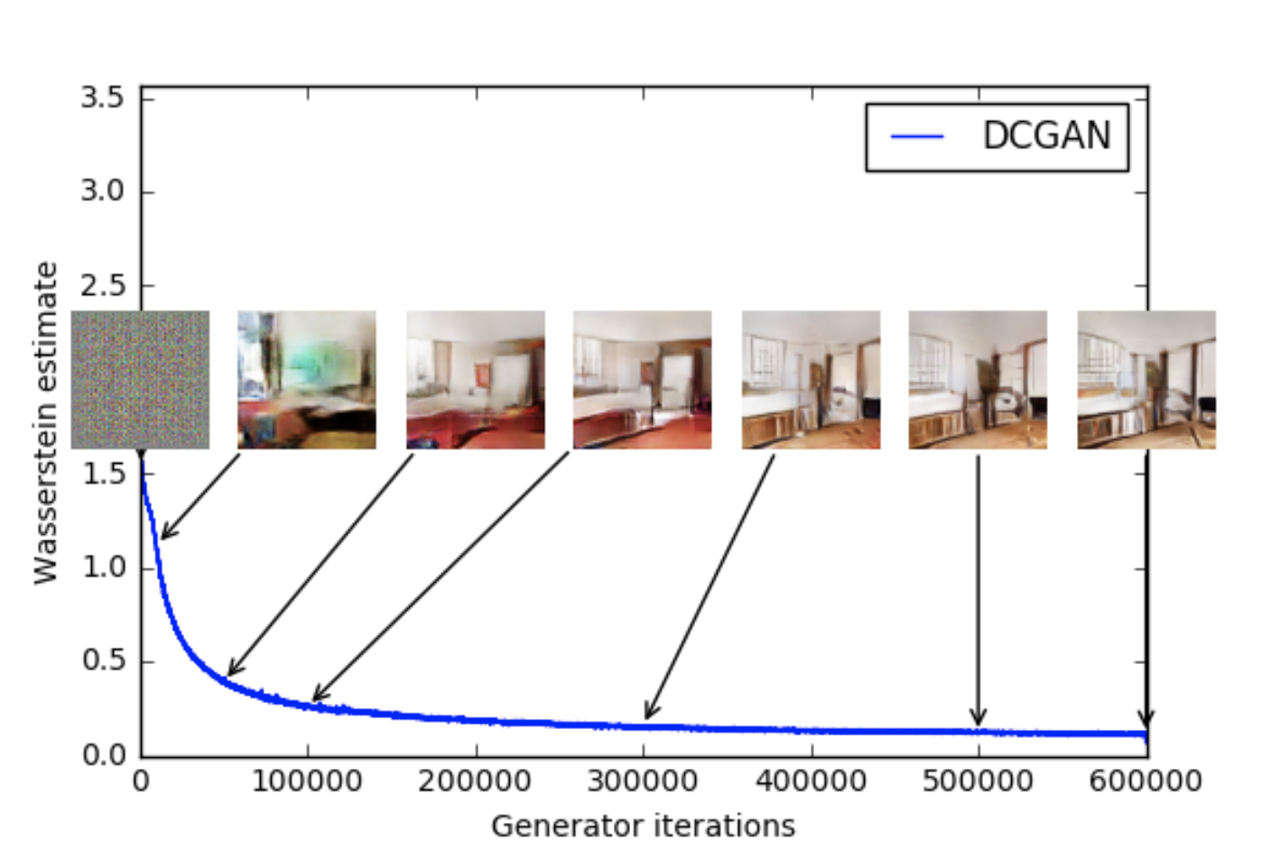 Figure 1: A WGAN with the DCGAN architecutre trained on the LSUN_Bedrooms dataset. As the Wasserstein Loss
goes down we see that the the sample quality gets better
Figure 1: A WGAN with the DCGAN architecutre trained on the LSUN_Bedrooms dataset. As the Wasserstein Loss
goes down we see that the the sample quality gets better
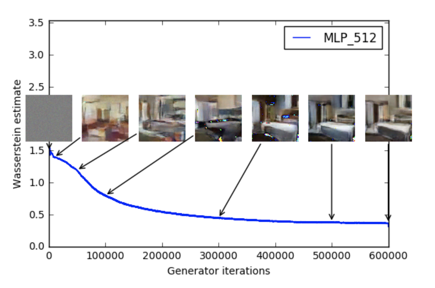 Figure 2: A WGAN with an MLP architecutre trained on the LSUN_Bedrooms dataset. As the Wasserstein Loss
goes down we see that the sample quality gets better
Figure 2: A WGAN with an MLP architecutre trained on the LSUN_Bedrooms dataset. As the Wasserstein Loss
goes down we see that the sample quality gets better
Code
Here the code released by the authors implementing WGANs using Pytorch. Volodymyr Kuleshov too has a neat implementation of WGANs in Tensorflow/Keras in this repo.
Further Reading
This post just scratches the surface of WGANs. I strongly recommend you to read the paper if you’d like to delve deeper into how WGANs work. Here is also an excellent post by Alex Irpan that expands a little bit on the math of WGANs that is glossed over in the paper.