ShahRukh Athar, Evgeny Burnaev and Victor Lempitsky

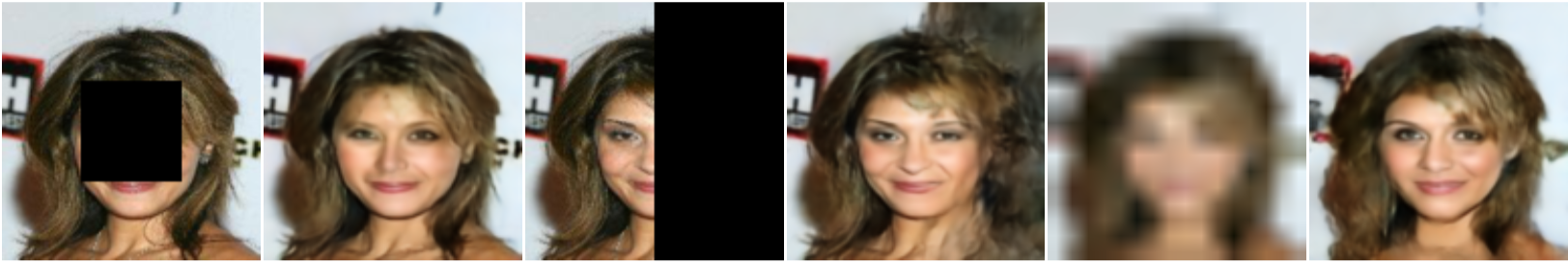_{Figure 1: Sample resotrations using a Latent Convolutional Model.}

Convolutional Neural Networks (CNN) have made a lasting impact on the entire field of computer vision with great results on segmentation, recognition and generative modelling of images. Of late, there has been an increasing amount of work [1,2] suggesting that the structure of the Convolutional Neural Network itself plays a rather important role in building unsupervised models of images and our work provides further evidence to support this claim. We present a new latent model of natural images that can be learned on large-scale datasets. The learning process provides a latent embedding for every image in the training dataset, as well as a generator network that maps each element of the latent space to the image space. The latent space our model uses is relatively high-dimensional and is parametrized by convolutional neural networks that are unique to each image. We call this latent space the convolutional manifold. In our experiments, we find that the convolutional manifold allows us to perform good quality image restoration from a wide variety of degradations at relatively high dimensions.

How does it work?

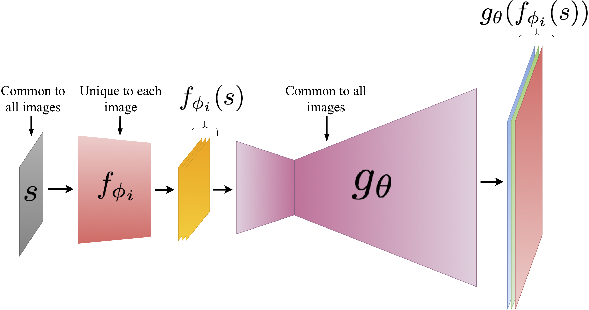_{Figure 2: The Schematic of a Latent Convolutional Model. The smaller CNN, \(f_{\phi}\) (red), is unique to each image and parametrizes the latent space of the generator, \(g_{\theta}\) (magenta), which is common to all images. The input \(s\) is fixed to random noise and is not updated during the training process.}

The convolutional manifold is central to the working of the Latent Convolutional Model (LCM), let’s start by describing what it is. Given a 3D map \(s\) of size \(W_{s}\times{}H_{s}\times{}C_{s}\) and a set of convolutional networks \(\{f_{\phi} |\ \phi \in \Phi\}\) of the same architecture, \(f\), the convolutional manifold \(\mathbb{C}_{f,s}\) is defined as

Various choices of \(\phi \in \Phi\) span the manifold for a given architecture \(f\), \(s\) and \(\Phi\). In our work, we have chosen \(s\) to be a map filled with uniform noise, \(f\) to be a CNN with 4 or 5 layers and \(\Phi= [-B, B]^{N_{\phi}}\) where \(N_{\phi}\) is the number of parameters in \(f\) and \(B\) is some constant value. The convolutional manifold was inspired by the work done in [2] where the authors effectively use it to model images in the image-space itself. In contrast, we use the convolutional manifold to model a latent space of images that can mapped to the image space using a generator network, thus allowing us to learn a latent representation of any given dataset of images. The work done in [2] showed that the regularization imposed by the structure of a CNN is quite helpful while modelling images and we intuit that a similar regularization would also be helpful while learning high dimensional latent space models.

The training process of an LCM, which is largely inspired by [1], works by jointly training a generator, \(g_{\theta}\), and the “latent” CNNs, \(f_{\phi_{i}}\)’s, that are unique to each image. Given a dataset of images \(\mathcal{D} = \{x_{1}, x_{2}, ..., x_{M}\}\) from some distribution \(\mathcal{X}\), we pair with each image \(x_{i}\), a latent CNN \(f_{\phi_{i}}\) with parameters \(\phi_{i}\) and some architecture \(f\). We now jointly optimize the \(\phi_{i}\)’s and the parameters \(\theta\) of a generator \(g_{\theta}\) for a minibatch of size \(N\) as follows

with additional constraints that \(\phi_{i} \in [-0.01, 0.01]\). The loss function we use is the Laplacian-L1: \(\mathcal{L}(x_{1},x_{2})_\text{Lap-L1} = \sum_{j}2^{-2j}|L^{j}(x_{1} - x_{2})|_{1}\) where \(L^{j}\) is the \(j\)th level of the Laplacian image pyramid. To speed up convergence during training we also add the MSE loss to the Lap-L1 term. We carry out the optimization above using vanilla stochastic gradient descent. As the model is learnt, each image, \(x_{i}\), gets a representation \(z_{i} = f_{\phi_{i}}(s)\) on the convolutional manifold. Further, each element in the convolutional manifold would define an image in the image-space:

Though not all elements in \(\mathbb{I}_{f,s,\theta}\) would belong to \(\mathcal{X}\), we found that the resulting manifold can cover \(\mathcal{X}\)’s support quite well with its each element having a very close approximation on \(\mathbb{I}_{f,s,\theta}\).

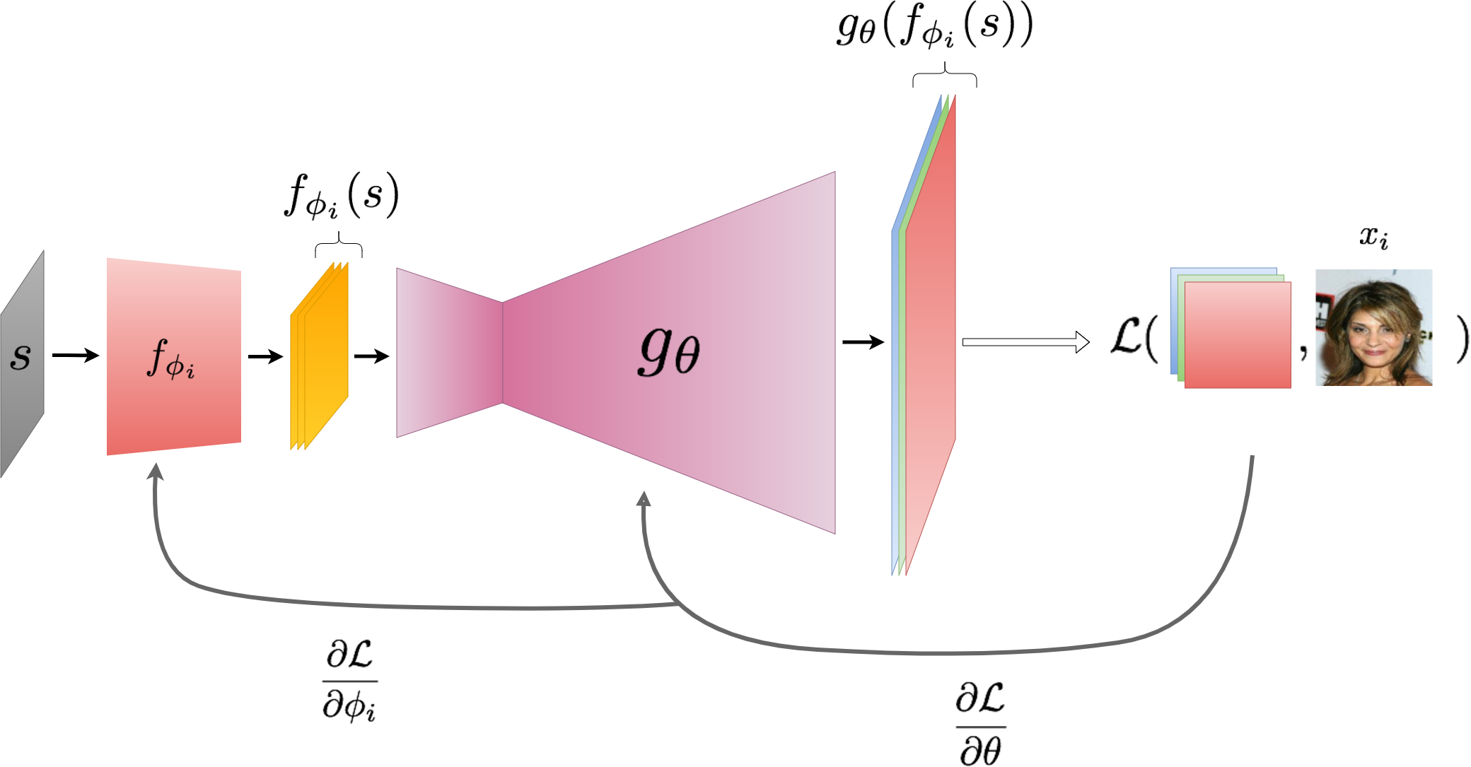_{Figure 3: Training an LCM. The parameters of the smaller CNN, \(f_{\phi}\) (red), and the generator, \(g_{\theta}\) (magenta), are minimized jointly. The input \(s\) is fixed to random noise and is not updated during the training process.}

Image Restoration using an LCM

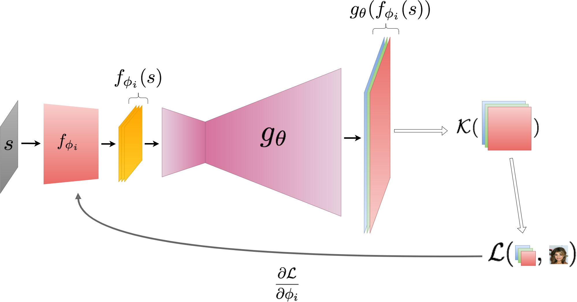_{Figure 4: Image super-resolution using an LCM. The parameters of the smaller CNN, \(f_{\phi}\) (red), are updated to match the downsampled image while the paramters of the generator, \(g_{\theta}\) (magenta), and the input \(s\) are kept fixed. Here \(\mathcal{K}\) is the downsampling kernel.}

For any given degrading transformation \(\mathcal{T}\) - which can be multiplication with a binary mask for inpainting, the downsampling kernel for super-resolution or graying for colorization - we carry out the following optimization to restore images

Here \(g\) is the generator that outputs the image, \(\omega\) are the relevant parameters in the latent space to optimize over and \(\mathcal{L}\) is the Lap-L1 and MSE loss. Figure 4 gives a schematic of super-resolving images using an LCM. Figures 5 and 6 show qualitative and quantitative results of inpainting, super-resolution and colorization using an LCM on the CelebA dataset at a resolution of \(128\times{}128\). Perceptual metrics and results on more datasets can be found in the paper and the supplementary material.

_{Figure 5: Inpainting, Super-Resolution and Colorization results on CelebA at \(128\times{}128\) resolution. The compared models are Generative Latent Space Optimization (GLO) [1], Deep Image Prior (DIP) [2], Wasserstein GAN with Gradient Penalty (WGAN) [3] and Autoencoders (AE) [4].}

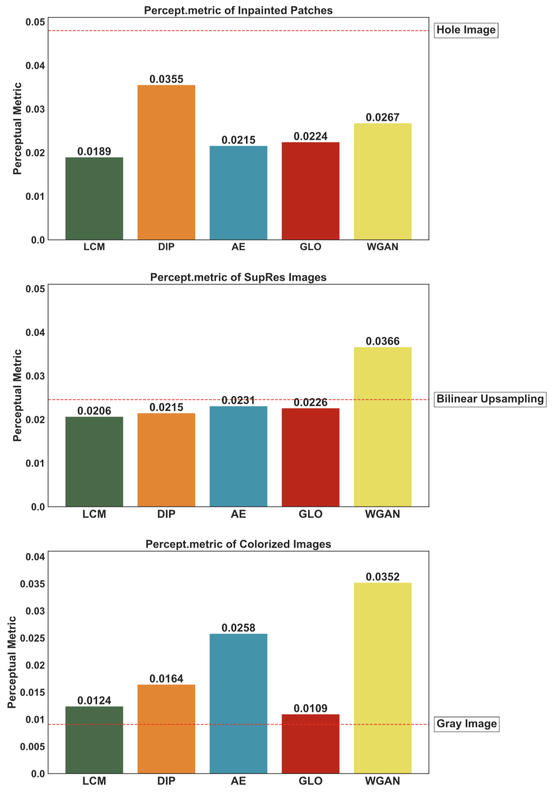_{Figure 6: Perceptual metrics of the various restorations on CelebA at \(128\times{}128\) resolution. The compared models are Generative Latent Space Optimization (GLO) [1], Deep Image Prior (DIP) [2], Wasserstein GAN with Gradient Penalty (WGAN) [3] and Autoencoders (AE) [4].}

Citation

@INPROCEEDINGS{LCMAthar2019,
  author = {ShahRukh Athar and Evgeny Burnaev and Victor Lempitsky},
  title = {Latent Convolutional Models},
  booktitle = {International Conference on Learning Representations (ICLR)},
  year = {2019}
}

Additional Resources

• Code
• Paper

References

• [1] P. Bojanowski, A. Joulin, D. Lopez-Paz, and A. Szlam. Optimizing the latent space of generative networks. In Proc. ICML, 2018.
• [2] D. Ulyanov, A. Vedaldi, and V. Lempitsky. Deep image prior. In Proc. CVPR, 2018.
• [3] Ishaan Gulrajani, Faruk Ahmed, Martin Arjovsky, Vincent Dumoulin, and Aaron C Courville. Improved training of Wasserstein GANs. In Proc. NIPS, 2017.
• [4] Ian Goodfellow, Yoshua Bengio, and Aaron Courville. Deep Learning. MIT Press, 2016.